
Improving DAX measure speed. We can take a measure like the one customer order measure, add it to a card visual, and use the performance analyser to give us the DAX query, which we can paste into the performance analyser. However, we may see different results if we use it in a matrix, so we will test that too.
The original DAX measure is as follows, and the test measures are found here, which use different functions to create the virtual tables used in the methods. The first measure is below, and we will look at the output of the server timings in more detail, using AI to help us analyse the output.
You can download DAX Studio here
DAX measure Code example to be used for improving DAX measure speed
CustomersWithOneOrder =
VAR _CustomerOrders = SUMMARIZE('FactInternetSales', -- Table
                            'FactInternetSales'[CustomerKey], -- Groupby
                             "Orders", DISTINCTCOUNT('FactInternetSales'[SalesOrderNumber])
                                )
VAR _OneOrder = FILTER(_CustomerOrders, [Orders] = 1)

RETURN
COUNTROWS(_OneOrder)
The DAX query created by the Formula Engine (copied from the performance analyser) is as follows for a card visual (total only):
// DAX Query
EVALUATE
    ROW(
    "CustomersWithOneOrder", '_Measures'[CustomersWithOneOrder]
)
In DAX Studio, we can paste in the code, clear the cache first, select server time, and all the options to show us each step of the query plan
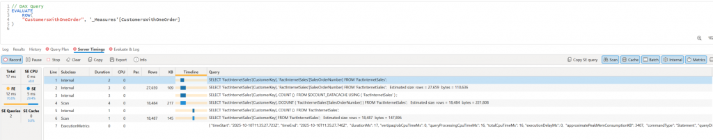
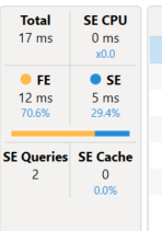
The first part of the server timings shows us that the query took 12 ms in the Formula engine (FE) and 5 ms in the storage engine (SE) a total of 12 ms to run. In addition, we can see that a total of 2 SE queries were parsed to the Vertipaq engine.
This SQL-like language is called xmlSQL and here are the steps that we can see in DAX Studio.
-- Line 1, Subclass Internal, Duration 2 rows 0
SET DC_KIND="GEC32"; -- Selecting distinct count strategy DC_KIND
SELECT
'FactInternetSales'[CustomerKey],
'FactInternetSales'[SalesOrderNumber]
FROM 'FactInternetSales';
-----------------------------------
Line 2, Subclass: Internal, Duration 3 rows 27,659 --- builds a datacache projects of the 2 columns it needs
SET DC_KIND="GEC32";
SELECT
'FactInternetSales'[CustomerKey],
'FactInternetSales'[SalesOrderNumber]
FROM 'FactInternetSales';
Estimated size: rows = 27,659 bytes = 110,636
---------------------------------
Line 3, Subclass: Internal, Duration 3, rows 0 ---use the disinct cache count from the data cached.
SET DC_KIND="C32";
SELECT
'FactInternetSales'[CustomerKey],
COUNT ()
FROM $DCOUNT_DATACACHE USING ( 'FactInternetSales' ) ;
----------------------------
Line 4, Subclass: Scan, Duration 4, Rows 18,484 --- this is the real storage engine scan with a DCOUNT aggregation, group by customerkey
SET DC_KIND="AUTO";
SELECT
'FactInternetSales'[CustomerKey],
DCOUNT ( 'FactInternetSales'[SalesOrderNumber] )
FROM 'FactInternetSales';
Estimated size: rows = 18,484 bytes = 221,808
------------------------------------------
Line 5, Subclass Internal, Duration 1, rows 0 --- auzillary count to help the optimizer (density/cardinatlity hints).
SET DC_KIND="DENSE";
SELECT
'FactInternetSales'[CustomerKey],
COUNT ()
FROM 'FactInternetSales';
------------------------------------------
Line 6, Subclass Scan, Duration 1, Rows 18,487 --another quick scan of customerkey likely to get the distinct key
SET DC_KIND="AUTO";
SELECT
'FactInternetSales'[CustomerKey]
FROM 'FactInternetSales';
Estimated size: rows = 18,487 bytes = 147,896
------------------------------------------
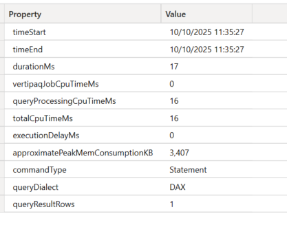
Line 7, Duration 0 refers to the execution metrics
Note that the actual result is 11619, which is not shown in the server timings. The server timings show the intermediary steps.
So that was all very interesting, but what do we do with it? Well, first, we can use it to compare measures as follows:
Card Visual (Total) DAX query performance
| Table function used in measures | FE | SE | Total | SE Queries | Approx. Peak Mem Consumption (Bytes) |
| SUMMARIZE() | 12 | 0 | 13 | 2 | 3407 |
| SELECTCOLUMS() | 10 | 7 | 17 | 2 | 2379 |
| SUMMARIZECOLUMNS() | 8 | 10 | 18 | 1 | 3376 |
| FILTER() | 6 | 7 | 13 | 1 | 3357 |
In the first test, which was based on the DAX query total on a card visual, all the measures ran very fast, with the summarize() and filter() functions performing faster. So based on this, we might run off and decide to use one of these, but then what if we want to use them in a different visual? Will the performance be the same?
Matrix Visual DAX Query performance
| Table function used in measures | FE | SE | Total | SE Queries | Approx. Peak Mem Consumption (Bytes) |
| Summarize() | 79 | 250 | 329 | 5 | 39,884 |
| Selectcolumns() | 41 | 49 | 90 | 6 | 11,968 |
| SummarizeColumns() | 19 | 26 | 45 | 3 | 99,54 |
| FILTER() | 24 | 73 | 97 | 5 | 10,445 |
So, as we can see, in the DAX query taken from the matrix test, the SUMMARIZE() function performed very poorly, with the measure that used the SUMMARIZECOLUMNS performing best. As you can see, this adds a whole different level of complexity to testing.
A solution for this is to use the ISINSCOPE() function to determine the scope of how the measure is being filtered and use it to switch between 2 different measures, but of course, that makes the model more complex and is a topic for another day.
We delve more deeply into performance optimisation with the post Dax Optimisation – Analysing the query plan and storage retrieval.