When jumping from one project to another, it can be useful to be able to compare common code structures.
I couldn’t find anything like this out there, so here it is magically created.
Contents:
Common Code Structures
Working with Dates
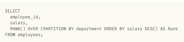
Window Functions
Error Handling
Casting
Joining Tables
CTE (Common Table Expressions)
Common Code Structures
| Topic | SQL Server | Snowflake | BigQuery |
|---|---|---|---|
| Select & Filtering | SELECT TOP 10 * FROM Sales WHERE Amount > 1000; |
SELECT * FROM Sales WHERE Amount > 1000 LIMIT 10; |
SELECT * FROM `project.dataset.Sales` WHERE Amount > 1000 LIMIT 10; |
| String Functions | SELECT LEFT(CustomerName, 5), LEN(CustomerName) FROM Customers; |
SELECT LEFT(CustomerName, 5), LENGTH(CustomerName) FROM Customers; |
SELECT SUBSTR(CustomerName, 1, 5), LENGTH(CustomerName) FROM `project.dataset.Customers`; |
| Date Functions | SELECT GETDATE() AS CurrentDate, DATEADD(DAY, 7, GETDATE()); |
SELECT CURRENT_DATE, DATEADD(DAY, 7, CURRENT_DATE); |
SELECT CURRENT_DATE(), DATE_ADD(CURRENT_DATE(), INTERVAL 7 DAY); |
| Joins | SELECT c.CustomerName, o.OrderID FROM Customers c INNER JOIN Orders o ON c.CustomerID = o.CustomerID; |
SELECT c.CustomerName, o.OrderID FROM Customers c JOIN Orders o ON c.CustomerID = o.CustomerID; |
SELECT c.CustomerName, o.OrderID FROM `project.dataset.Customers` c JOIN `project.dataset.Orders` o ON c.CustomerID = o.CustomerID; |
| Aggregations & Group By | SELECT CustomerID, SUM(Amount) AS TotalAmount FROM Sales GROUP BY CustomerID HAVING SUM(Amount) > 1000; |
SELECT CustomerID, SUM(Amount) AS TotalAmount FROM Sales GROUP BY CustomerID HAVING SUM(Amount) > 1000; |
SELECT CustomerID, SUM(Amount) AS TotalAmount FROM `project.dataset.Sales` GROUP BY CustomerID HAVING SUM(Amount) > 1000; |
| Window Functions | SELECT CustomerID,
SUM(Amount) OVER (PARTITION BY CustomerID) AS TotalByCustomer
FROM Sales; |
SELECT CustomerID,
       SUM(Amount) OVER (PARTITION BY CustomerID) AS TotalByCustomer
FROM Sales; |
SELECT CustomerID,
       SUM(Amount) OVER (PARTITION BY CustomerID) AS TotalByCustomer
FROM `project.dataset.Sales`; |
| Creating Tables | CREATE TABLE Customers (
CustomerID INT PRIMARY KEY,
CustomerName NVARCHAR(100)
); |
CREATE TABLE Customers (
    CustomerID INT PRIMARY KEY,
    CustomerName STRING
); |
CREATE TABLE dataset.Customers (
    CustomerID INT64,
    CustomerName STRING
); |
| Insert | INSERT INTO Customers (CustomerID, CustomerName) VALUES (1, 'John Doe'); |
INSERT INTO Customers (CustomerID, CustomerName) VALUES (1, 'John Doe'); |
INSERT INTO dataset.Customers (CustomerID, CustomerName) VALUES (1, 'John Doe'); |
| Update | UPDATE Customers SET CustomerName = 'Jane Doe' WHERE CustomerID = 1; |
UPDATE Customers SET CustomerName = 'Jane Doe' WHERE CustomerID = 1; |
UPDATE dataset.Customers SET CustomerName = 'Jane Doe' WHERE CustomerID = 1; |
| Delete | DELETE FROM Customers WHERE CustomerID = 1; |
DELETE FROM Customers WHERE CustomerID = 1; |
DELETE FROM dataset.Customers WHERE CustomerID = 1; |
| Case When Statements | SELECT OrderID,
CASE
WHEN Amount >= 1000 THEN 'High'
WHEN Amount >= 500 THEN 'Medium'
ELSE 'Low'
END AS OrderCategory
FROM Sales; |
SELECT OrderID,
       CASE
         WHEN Amount >= 1000 THEN 'High'
         WHEN Amount >= 500  THEN 'Medium'
         ELSE 'Low'
       END AS OrderCategory
FROM Sales; |
SELECT OrderID,
       CASE
         WHEN Amount >= 1000 THEN 'High'
         WHEN Amount >= 500  THEN 'Medium'
         ELSE 'Low'
       END AS OrderCategory
FROM `project.dataset.Sales`; |
| Start of Month | SELECT OrderDate,
DATEADD(MONTH, DATEDIFF(MONTH, 0, OrderDate), 0) AS StartOfMonth
FROM Orders; |
SELECT OrderDate,
       DATE_TRUNC('MONTH', OrderDate) AS StartOfMonth
FROM Orders; |
SELECT OrderDate,
       DATE_TRUNC(OrderDate, MONTH) AS StartOfMonth
FROM `project.dataset.Orders`; |
| End of Month | SELECT OrderDate,
EOMONTH(OrderDate) AS EndOfMonth
FROM Orders; |
SELECT OrderDate,
       LAST_DAY(OrderDate, 'MONTH') AS EndOfMonth
FROM Orders; |
SELECT OrderDate,
       LAST_DAY(OrderDate, MONTH) AS EndOfMonth
FROM `project.dataset.Orders`; |
| Null Handling | SELECT CustomerID,
COALESCE(CustomerName, 'Unknown') AS SafeName
FROM Customers; |
SELECT CustomerID,
       COALESCE(CustomerName, 'Unknown') AS SafeName
FROM Customers; |
SELECT CustomerID,
       COALESCE(CustomerName, 'Unknown') AS SafeName
FROM `project.dataset.Customers`; |
| Conditional Aggregation | SELECT CustomerID,
SUM(CASE WHEN Amount > 1000 THEN Amount ELSE 0 END) AS HighValueSales
FROM Sales
GROUP BY CustomerID; |
SELECT CustomerID,
       SUM(CASE WHEN Amount > 1000 THEN Amount ELSE 0 END) AS HighValueSales
FROM Sales
GROUP BY CustomerID; |
SELECT CustomerID,
       SUM(CASE WHEN Amount > 1000 THEN Amount ELSE 0 END) AS HighValueSales
FROM `project.dataset.Sales`
GROUP BY CustomerID; |
| Date Difference | SELECT OrderID,
DATEDIFF(DAY, OrderDate, ShippedDate) AS DaysToShip
FROM Orders; |
SELECT OrderID,
       DATEDIFF(DAY, OrderDate, ShippedDate) AS DaysToShip
FROM Orders; |
SELECT OrderID,
       DATE_DIFF(ShippedDate, OrderDate, DAY) AS DaysToShip
FROM `project.dataset.Orders`; |
Working with Dates
| Date Topic | SQL Server | Snowflake | BigQuery |
|---|---|---|---|
| Build Date from Parts | SELECT DATEFROMPARTS(2025, 10, 3) AS d; |
SELECT DATE_FROM_PARTS(2025, 10, 3) AS d; |
SELECT DATE(2025, 10, 3) AS d; |
| Parse Date from String | SELECT TRY_CONVERT(date, '03/10/2025', 103); -- DD/MM/YYYY SELECT CONVERT(date, '2025-10-03', 23); -- ISO |
SELECT TO_DATE('03/10/2025', 'DD/MM/YYYY');
SELECT TO_DATE('2025-10-03'); |
SELECT PARSE_DATE('%d/%m/%Y','03/10/2025');
SELECT DATE '2025-10-03'; |
| Current Date / Timestamp | SELECT CAST(GETDATE() AS date) AS current_date,
GETDATE() AS current_datetime; |
SELECT CURRENT_DATE AS current_date,
CURRENT_TIMESTAMP AS current_ts; |
SELECT CURRENT_DATE() AS current_date,
CURRENT_TIMESTAMP() AS current_ts; |
| Start of Month | SELECT DATEADD(MONTH, DATEDIFF(MONTH, 0, OrderDate), 0) FROM Orders; |
SELECT DATE_TRUNC('MONTH', OrderDate)
FROM Orders; |
SELECT DATE_TRUNC(OrderDate, MONTH) FROM `project.dataset.Orders`; |
| End of Month | SELECT EOMONTH(OrderDate) FROM Orders; |
SELECT LAST_DAY(OrderDate, 'MONTH') FROM Orders; |
SELECT LAST_DAY(OrderDate, MONTH) FROM `project.dataset.Orders`; |
| Add Days | SELECT DATEADD(DAY, 7, OrderDate) FROM Orders; |
SELECT DATEADD(DAY, 7, OrderDate) FROM Orders; |
SELECT DATE_ADD(OrderDate, INTERVAL 7 DAY) FROM `project.dataset.Orders`; |
| Add Months | SELECT DATEADD(MONTH, 3, OrderDate) FROM Orders; |
SELECT DATEADD(MONTH, 3, OrderDate) FROM Orders; |
SELECT DATE_ADD(OrderDate, INTERVAL 3 MONTH) FROM `project.dataset.Orders`; |
| Difference (Days) | SELECT DATEDIFF(DAY, OrderDate, ShippedDate) FROM Orders; |
SELECT DATEDIFF('DAY', OrderDate, ShippedDate)
FROM Orders; |
SELECT DATE_DIFF(ShippedDate, OrderDate, DAY) FROM `project.dataset.Orders`; |
| Difference (Months) | SELECT DATEDIFF(MONTH, StartDate, EndDate) AS months_between; |
SELECT DATEDIFF('MONTH', StartDate, EndDate) AS months_between; |
SELECT DATE_DIFF(EndDate, StartDate, MONTH) AS months_between; |
| Truncate to Week (Week Start) | -- Week starting Sunday SELECT DATEADD(WEEK, DATEDIFF(WEEK, 0, OrderDate), 0) FROM Orders; |
-- ISO week (Mon start)
SELECT DATE_TRUNC('WEEK', OrderDate)
FROM Orders; |
-- Default WEEK (Sun). Use WEEK(MONDAY) if needed SELECT DATE_TRUNC(OrderDate, WEEK) FROM `project.dataset.Orders`; |
| Truncate to Quarter | SELECT DATEADD(QUARTER, DATEDIFF(QUARTER, 0, OrderDate), 0) FROM Orders; |
SELECT DATE_TRUNC('QUARTER', OrderDate)
FROM Orders; |
SELECT DATE_TRUNC(OrderDate, QUARTER) FROM `project.dataset.Orders`; |
| First Day of Year | SELECT DATEADD(YEAR, DATEDIFF(YEAR, 0, OrderDate), 0) FROM Orders; |
SELECT DATE_TRUNC('YEAR', OrderDate)
FROM Orders; |
SELECT DATE_TRUNC(OrderDate, YEAR) FROM `project.dataset.Orders`; |
| Last Day of Year | SELECT EOMONTH(DATEFROMPARTS(YEAR(OrderDate), 12, 1)) FROM Orders; |
SELECT LAST_DAY(OrderDate, 'YEAR') FROM Orders; |
SELECT LAST_DAY(OrderDate, YEAR) FROM `project.dataset.Orders`; |
| Extract Year / Month / Day | SELECT YEAR(OrderDate) AS y,
MONTH(OrderDate) AS m,
DAY(OrderDate) AS d
FROM Orders; |
SELECT YEAR(OrderDate) AS y,
       MONTH(OrderDate) AS m,
       DAY(OrderDate) AS d
FROM Orders; |
SELECT EXTRACT(YEAR FROM OrderDate) AS y,
       EXTRACT(MONTH FROM OrderDate) AS m,
       EXTRACT(DAY FROM OrderDate) AS d
FROM `project.dataset.Orders`; |
| Day Name / Weekday | SELECT DATENAME(WEEKDAY, OrderDate) AS day_name,
DATEPART(WEEKDAY, OrderDate) AS weekday_num
FROM Orders; |
SELECT DAYNAME(OrderDate) AS day_name,
       DAYOFWEEK(OrderDate) AS weekday_num
FROM Orders; |
SELECT FORMAT_DATE('%A', OrderDate) AS day_name,
       EXTRACT(DAYOFWEEK FROM OrderDate) AS weekday_num
FROM `project.dataset.Orders`; |
| Between Dates (Inclusive) | SELECT * FROM Orders WHERE OrderDate BETWEEN '2025-10-01' AND '2025-10-31'; |
SELECT * FROM Orders WHERE OrderDate BETWEEN '2025-10-01' AND '2025-10-31'; |
SELECT * FROM `project.dataset.Orders` WHERE OrderDate BETWEEN DATE '2025-10-01' AND DATE '2025-10-31'; |
| Last 30 Days Filter | SELECT * FROM Orders WHERE OrderDate >= DATEADD(DAY, -30, CAST(GETDATE() AS date)); |
SELECT * FROM Orders WHERE OrderDate >= DATEADD(DAY, -30, CURRENT_DATE); |
SELECT * FROM `project.dataset.Orders` WHERE OrderDate >= DATE_SUB(CURRENT_DATE(), INTERVAL 30 DAY); |
Window Functions
| Window Topic | SQL Server | Snowflake | BigQuery |
|---|---|---|---|
| Running Total | SELECT CustomerID, OrderDate, Amount,
SUM(Amount) OVER (
PARTITION BY CustomerID
ORDER BY OrderDate
ROWS BETWEEN UNBOUNDED PRECEDING AND CURRENT ROW
) AS RunningTotal
FROM Sales; |
SELECT CustomerID, OrderDate, Amount,
  SUM(Amount) OVER (
    PARTITION BY CustomerID
    ORDER BY OrderDate
    ROWS BETWEEN UNBOUNDED PRECEDING AND CURRENT ROW
  ) AS RunningTotal
FROM Sales; |
SELECT CustomerID, OrderDate, Amount,
  SUM(Amount) OVER (
    PARTITION BY CustomerID
    ORDER BY OrderDate
    ROWS BETWEEN UNBOUNDED PRECEDING AND CURRENT ROW
  ) AS RunningTotal
FROM `project.dataset.Sales`; |
| Moving Avg (7 rows) | SELECT OrderDate, Amount,
AVG(Amount) OVER (
ORDER BY OrderDate
ROWS BETWEEN 6 PRECEDING AND CURRENT ROW
) AS MovAvg7
FROM Sales; |
SELECT OrderDate, Amount,
  AVG(Amount) OVER (
    ORDER BY OrderDate
    ROWS BETWEEN 6 PRECEDING AND CURRENT ROW
  ) AS MovAvg7
FROM Sales; |
SELECT OrderDate, Amount,
  AVG(Amount) OVER (
    ORDER BY OrderDate
    ROWS BETWEEN 6 PRECEDING AND CURRENT ROW
  ) AS MovAvg7
FROM `project.dataset.Sales`; |
| ROW_NUMBER | SELECT *,
ROW_NUMBER() OVER (
PARTITION BY CustomerID ORDER BY OrderDate DESC
) AS rn
FROM Sales; |
SELECT *,
  ROW_NUMBER() OVER (
    PARTITION BY CustomerID ORDER BY OrderDate DESC
  ) AS rn
FROM Sales; |
SELECT *,
  ROW_NUMBER() OVER (
    PARTITION BY CustomerID ORDER BY OrderDate DESC
  ) AS rn
FROM `project.dataset.Sales`; |
| RANK | SELECT CustomerID, Amount, RANK() OVER (PARTITION BY CustomerID ORDER BY Amount DESC) AS rnk FROM Sales; |
SELECT CustomerID, Amount, RANK() OVER (PARTITION BY CustomerID ORDER BY Amount DESC) AS rnk FROM Sales; |
SELECT CustomerID, Amount, RANK() OVER (PARTITION BY CustomerID ORDER BY Amount DESC) AS rnk FROM `project.dataset.Sales`; |
| DENSE_RANK | SELECT CustomerID, Amount, DENSE_RANK() OVER (PARTITION BY CustomerID ORDER BY Amount DESC) AS drnk FROM Sales; |
SELECT CustomerID, Amount, DENSE_RANK() OVER (PARTITION BY CustomerID ORDER BY Amount DESC) AS drnk FROM Sales; |
SELECT CustomerID, Amount, DENSE_RANK() OVER (PARTITION BY CustomerID ORDER BY Amount DESC) AS drnk FROM `project.dataset.Sales`; |
| NTILE (Quartiles) | SELECT CustomerID, Amount, NTILE(4) OVER (ORDER BY Amount DESC) AS quartile FROM Sales; |
SELECT CustomerID, Amount, NTILE(4) OVER (ORDER BY Amount DESC) AS quartile FROM Sales; |
SELECT CustomerID, Amount, NTILE(4) OVER (ORDER BY Amount DESC) AS quartile FROM `project.dataset.Sales`; |
| LAG (Prev Row) | SELECT OrderDate, Amount, LAG(Amount, 1) OVER (ORDER BY OrderDate) AS PrevAmt FROM Sales; |
SELECT OrderDate, Amount, LAG(Amount, 1) OVER (ORDER BY OrderDate) AS PrevAmt FROM Sales; |
SELECT OrderDate, Amount, LAG(Amount, 1) OVER (ORDER BY OrderDate) AS PrevAmt FROM `project.dataset.Sales`; |
| LEAD (Next Row) | SELECT OrderDate, Amount, LEAD(Amount, 1) OVER (ORDER BY OrderDate) AS NextAmt FROM Sales; |
SELECT OrderDate, Amount, LEAD(Amount, 1) OVER (ORDER BY OrderDate) AS NextAmt FROM Sales; |
SELECT OrderDate, Amount, LEAD(Amount, 1) OVER (ORDER BY OrderDate) AS NextAmt FROM `project.dataset.Sales`; |
| FIRST_VALUE | SELECT OrderDate, Amount,
FIRST_VALUE(Amount) OVER (
ORDER BY OrderDate
ROWS BETWEEN UNBOUNDED PRECEDING AND CURRENT ROW
) AS FirstAmt
FROM Sales; |
SELECT OrderDate, Amount,
  FIRST_VALUE(Amount) OVER (
    ORDER BY OrderDate
    ROWS BETWEEN UNBOUNDED PRECEDING AND CURRENT ROW
  ) AS FirstAmt
FROM Sales; |
SELECT OrderDate, Amount,
  FIRST_VALUE(Amount) OVER (
    ORDER BY OrderDate
    ROWS BETWEEN UNBOUNDED PRECEDING AND CURRENT ROW
  ) AS FirstAmt
FROM `project.dataset.Sales`; |
| LAST_VALUE* | SELECT OrderDate, Amount,
LAST_VALUE(Amount) OVER (
ORDER BY OrderDate
ROWS BETWEEN UNBOUNDED PRECEDING AND UNBOUNDED FOLLOWING
) AS LastAmt
FROM Sales; |
SELECT OrderDate, Amount,
  LAST_VALUE(Amount) OVER (
    ORDER BY OrderDate
    ROWS BETWEEN UNBOUNDED PRECEDING AND UNBOUNDED FOLLOWING
  ) AS LastAmt
FROM Sales; |
SELECT OrderDate, Amount,
  LAST_VALUE(Amount) OVER (
    ORDER BY OrderDate
    ROWS BETWEEN UNBOUNDED PRECEDING AND UNBOUNDED FOLLOWING
  ) AS LastAmt
FROM `project.dataset.Sales`; |
| PERCENT_RANK() | SELECT Amount, PERCENT_RANK() OVER (ORDER BY Amount) AS pct_rank FROM Sales; |
SELECT Amount, PERCENT_RANK() OVER (ORDER BY Amount) AS pct_rank FROM Sales; |
SELECT Amount, PERCENT_RANK() OVER (ORDER BY Amount) AS pct_rank FROM `project.dataset.Sales`; |
| CUME_DIST() | SELECT Amount, CUME_DIST() OVER (ORDER BY Amount) AS cume FROM Sales; |
SELECT Amount, CUME_DIST() OVER (ORDER BY Amount) AS cume FROM Sales; |
SELECT Amount, CUME_DIST() OVER (ORDER BY Amount) AS cume FROM `project.dataset.Sales`; |
| Share of Total | SELECT CustomerID, Amount,
Amount * 1.0 / SUM(Amount) OVER (
PARTITION BY CustomerID
) AS ShareOfCust
FROM Sales; |
SELECT CustomerID, Amount,
  Amount / SUM(Amount) OVER (
    PARTITION BY CustomerID
  ) AS ShareOfCust
FROM Sales; |
SELECT CustomerID, Amount,
  Amount / SUM(Amount) OVER (
    PARTITION BY CustomerID
  ) AS ShareOfCust
FROM `project.dataset.Sales`; |
| COUNT Over Window | SELECT CustomerID, OrderDate,
COUNT(*) OVER (
PARTITION BY CustomerID
ORDER BY OrderDate
ROWS BETWEEN UNBOUNDED PRECEDING AND CURRENT ROW
) AS CntToDate
FROM Sales; |
SELECT CustomerID, OrderDate,
  COUNT(*) OVER (
    PARTITION BY CustomerID
    ORDER BY OrderDate
    ROWS BETWEEN UNBOUNDED PRECEDING AND CURRENT ROW
  ) AS CntToDate
FROM Sales; |
SELECT CustomerID, OrderDate,
  COUNT(*) OVER (
    PARTITION BY CustomerID
    ORDER BY OrderDate
    ROWS BETWEEN UNBOUNDED PRECEDING AND CURRENT ROW
  ) AS CntToDate
FROM `project.dataset.Sales`; |
| Distinct Count in Window | -- COUNT(DISTINCT) OVER is not supported.
-- Workaround: distinct per partition via DENSE_RANK.
WITH x AS (
SELECT CustomerID, ProductID,
DENSE_RANK() OVER (
PARTITION BY CustomerID ORDER BY ProductID
) AS r
FROM Sales
)
SELECT CustomerID, MAX(r) AS DistinctProducts
FROM x GROUP BY CustomerID; |
-- COUNT(DISTINCT) OVER not supported in Snowflake windows. -- Use DENSE_RANK or COUNT(DISTINCT) without OVER at final grouping. |
-- COUNT(DISTINCT) OVER not supported in BigQuery windows. -- Use DENSE_RANK or COUNT(DISTINCT) at GROUP BY level. |
Error Handling
| Error Handling Topic | SQL Server | Snowflake | BigQuery |
|---|---|---|---|
| Replace NULL with Default | SELECT ISNULL(Amount, 0) AS SafeAmt,
COALESCE(CustomerName, 'Unknown') AS SafeName
FROM Sales; |
SELECT IFNULL(Amount, 0) AS SafeAmt,
       COALESCE(CustomerName, 'Unknown') AS SafeName
FROM Sales; |
SELECT IFNULL(Amount, 0) AS SafeAmt,
       COALESCE(CustomerName, 'Unknown') AS SafeName
FROM `project.dataset.Sales`; |
| Safe Division by Zero | SELECT CASE WHEN Denominator = 0
THEN NULL
ELSE Numerator * 1.0 / Denominator END AS Ratio
FROM Data; |
SELECT DIV0(Numerator, Denominator) AS Ratio FROM Data; |
SELECT SAFE_DIVIDE(Numerator, Denominator) AS Ratio FROM `project.dataset.Data`; |
| Safe Cast / Conversion | SELECT TRY_CAST(Value AS INT) AS SafeInt FROM RawData; |
SELECT TRY_TO_NUMBER(Value) AS SafeInt FROM RawData; |
SELECT SAFE_CAST(Value AS INT64) AS SafeInt FROM `project.dataset.RawData`; |
| Null If | SELECT NULLIF(Amount, 0) AS NullIfZero FROM Sales; |
SELECT NULLIF(Amount, 0) AS NullIfZero FROM Sales; |
SELECT NULLIF(Amount, 0) AS NullIfZero FROM `project.dataset.Sales`; |
| Error Catch / Try | BEGIN TRY SELECT 1/0; END TRY BEGIN CATCH SELECT ERROR_MESSAGE(); END CATCH; |
-- Snowflake doesn’t have TRY/CATCH in SQL. -- Use TRY_* functions (TRY_TO_NUMBER, TRY_CAST) to avoid errors. |
-- BigQuery doesn’t support TRY/CATCH in SQL. -- Use SAFE_CAST, SAFE_DIVIDE, IFERROR(expr, alt) in some contexts. |
| IfError Style (Return fallback if error) | -- Not native in T-SQL. -- Wrap in TRY/CATCH or use CASE + TRY_CAST. |
SELECT TRY_TO_NUMBER(Value, 0) AS SafeVal; |
SELECT IFERROR(1/0, NULL) AS SafeVal; |
Casting
| Casting Topic | SQL Server | Snowflake | BigQuery |
|---|---|---|---|
| Basic CAST | SELECT CAST(Amount AS DECIMAL(12,2)) AS amt_dec; |
SELECT CAST(Amount AS NUMBER(12,2)) AS amt_dec; |
SELECT CAST(Amount AS NUMERIC(12,2)) AS amt_dec; |
| Alt Syntax | SELECT CONVERT(DECIMAL(12,2), Amount) AS amt_dec; |
SELECT Amount::NUMBER(12,2) AS amt_dec; |
-- Standard CAST only (no ::) SELECT CAST(Amount AS NUMERIC(12,2)); |
| Safe Cast | SELECT TRY_CAST(Value AS INT) AS safe_int; |
SELECT TRY_TO_NUMBER(Value) AS safe_num; |
SELECT SAFE_CAST(Value AS INT64) AS safe_int; |
| String → INT | SELECT TRY_CONVERT(INT, '123') AS i; |
SELECT TRY_TO_NUMBER('123')::INT AS i; |
SELECT SAFE_CAST('123' AS INT64) AS i; |
| String → DECIMAL | SELECT TRY_CAST('123.45' AS DECIMAL(10,2)) AS d; |
SELECT TRY_TO_DECIMAL('123.45',10,2) AS d; |
SELECT SAFE_CAST('123.45' AS NUMERIC(10,2)) AS d; |
| String → DATE (format) | -- DD/MM/YYYY SELECT TRY_CONVERT(date, '03/10/2025', 103); |
SELECT TO_DATE('03/10/2025','DD/MM/YYYY'); |
SELECT PARSE_DATE('%d/%m/%Y', '03/10/2025'); |
| String → TIMESTAMP | SELECT TRY_CONVERT(datetime2, '2025-10-03T14:05:00Z', 127); |
SELECT TO_TIMESTAMP_TZ('2025-10-03T14:05:00Z'); |
SELECT TIMESTAMP('2025-10-03T14:05:00Z'); |
| Epoch Seconds → TS | SELECT DATEADD(SECOND, 1696341900, '1970-01-01'); |
SELECT TO_TIMESTAMP(1696341900); -- seconds |
SELECT TIMESTAMP_SECONDS(1696341900); |
| Time Zone Convert | SELECT (YourDT AT TIME ZONE 'UTC')
AT TIME ZONE 'Europe/Malta' AS local_dt; |
SELECT CONVERT_TIMEZONE('UTC','Europe/Malta', YourTS) AS local_ts; |
-- Convert UTC timestamp to Europe/Malta datetime SELECT DATETIME(TIMESTAMP(YourDT), 'Europe/Malta') AS local_dt; |
| String → BOOLEAN | -- No direct parse; map via CASE
SELECT CASE WHEN LOWER(val) IN ('true','1','y','yes') THEN 1 ELSE 0 END AS bitval; |
SELECT TRY_TO_BOOLEAN(val) AS b; |
SELECT SAFE_CAST(val AS BOOL) AS b; |
| To String (format) | SELECT CONVERT(varchar(10), OrderDate, 23) AS iso_date; -- YYYY-MM-DD |
SELECT TO_VARCHAR(OrderDate, 'YYYY-MM-DD') AS iso_date; |
SELECT FORMAT_DATE('%F', OrderDate) AS iso_date; |
| String → JSON | -- No JSON type. Keep NVARCHAR, use OPENJSON to shred: SELECT * FROM OPENJSON(@json); |
SELECT PARSE_JSON('{"a":1,"b":"x"}') AS j; -- VARIANT |
SELECT PARSE_JSON('{"a":1,"b":"x"}') AS j;  -- JSON
-- Safe variant:
SELECT SAFE.PARSE_JSON(json_str) AS j; |
| Any → JSON String | -- Build JSON via FOR JSON: SELECT * FROM T FOR JSON AUTO; |
SELECT TO_JSON(OBJECT_CONSTRUCT('a',1,'b','x')) AS json_s; |
SELECT TO_JSON(STRUCT(1 AS a, 'x' AS b)) AS json_s; |
| Date/Time Families | -- date, datetime, datetime2, time, smalldatetime |
-- DATE, TIME, TIMESTAMP_NTZ/LTZ/TTZ |
-- DATE, DATETIME, TIME, TIMESTAMP |
Joining Tables
| Join Type | SQL Server | Snowflake | BigQuery |
|---|---|---|---|
| INNER JOIN | SELECT c.CustomerName, o.OrderID FROM Customers c INNER JOIN Orders o ON c.CustomerID = o.CustomerID; |
SELECT c.CustomerName, o.OrderID FROM Customers c JOIN Orders o ON c.CustomerID = o.CustomerID; |
SELECT c.CustomerName, o.OrderID FROM `project.dataset.Customers` c JOIN `project.dataset.Orders` o ON c.CustomerID = o.CustomerID; |
| LEFT JOIN | SELECT c.CustomerName, o.OrderID FROM Customers c LEFT JOIN Orders o ON c.CustomerID = o.CustomerID; |
SELECT c.CustomerName, o.OrderID FROM Customers c LEFT JOIN Orders o ON c.CustomerID = o.CustomerID; |
SELECT c.CustomerName, o.OrderID FROM `project.dataset.Customers` c LEFT JOIN `project.dataset.Orders` o ON c.CustomerID = o.CustomerID; |
| RIGHT JOIN | SELECT c.CustomerName, o.OrderID FROM Customers c RIGHT JOIN Orders o ON c.CustomerID = o.CustomerID; |
SELECT c.CustomerName, o.OrderID FROM Customers c RIGHT JOIN Orders o ON c.CustomerID = o.CustomerID; |
SELECT c.CustomerName, o.OrderID FROM `project.dataset.Customers` c RIGHT JOIN `project.dataset.Orders` o ON c.CustomerID = o.CustomerID; |
| FULL OUTER JOIN | SELECT c.CustomerName, o.OrderID FROM Customers c FULL OUTER JOIN Orders o ON c.CustomerID = o.CustomerID; |
SELECT c.CustomerName, o.OrderID FROM Customers c FULL OUTER JOIN Orders o ON c.CustomerID = o.CustomerID; |
SELECT c.CustomerName, o.OrderID FROM `project.dataset.Customers` c FULL OUTER JOIN `project.dataset.Orders` o ON c.CustomerID = o.CustomerID; |
| CROSS JOIN | SELECT c.CustomerName, p.ProductName FROM Customers c CROSS JOIN Products p; |
SELECT c.CustomerName, p.ProductName FROM Customers c CROSS JOIN Products p; |
SELECT c.CustomerName, p.ProductName FROM `project.dataset.Customers` c CROSS JOIN `project.dataset.Products` p; |
| SELF JOIN | SELECT e1.EmployeeName, e2.ManagerName FROM Employees e1 JOIN Employees e2 ON e1.ManagerID = e2.EmployeeID; |
SELECT e1.EmployeeName, e2.ManagerName FROM Employees e1 JOIN Employees e2 ON e1.ManagerID = e2.EmployeeID; |
SELECT e1.EmployeeName, e2.ManagerName FROM `project.dataset.Employees` e1 JOIN `project.dataset.Employees` e2 ON e1.ManagerID = e2.EmployeeID; |
| Semi Join (Exists) | SELECT c.CustomerName FROM Customers c WHERE EXISTS ( SELECT 1 FROM Orders o WHERE o.CustomerID = c.CustomerID ); |
SELECT c.CustomerName FROM Customers c WHERE EXISTS ( SELECT 1 FROM Orders o WHERE o.CustomerID = c.CustomerID ); |
SELECT c.CustomerName FROM `project.dataset.Customers` c WHERE EXISTS ( SELECT 1 FROM `project.dataset.Orders` o WHERE o.CustomerID = c.CustomerID ); |
| Anti Join (Not Exists) | SELECT c.CustomerName FROM Customers c WHERE NOT EXISTS ( SELECT 1 FROM Orders o WHERE o.CustomerID = c.CustomerID ); |
SELECT c.CustomerName FROM Customers c WHERE NOT EXISTS ( SELECT 1 FROM Orders o WHERE o.CustomerID = c.CustomerID ); |
SELECT c.CustomerName FROM `project.dataset.Customers` c WHERE NOT EXISTS ( SELECT 1 FROM `project.dataset.Orders` o WHERE o.CustomerID = c.CustomerID ); |
CTE
| CTE Topic | SQL Server | Snowflake | BigQuery |
|---|---|---|---|
| Basic CTE | WITH TopSales AS ( SELECT CustomerID, Amount FROM Sales WHERE Amount > 1000 ) SELECT * FROM TopSales; |
WITH TopSales AS ( SELECT CustomerID, Amount FROM Sales WHERE Amount > 1000 ) SELECT * FROM TopSales; |
WITH TopSales AS ( SELECT CustomerID, Amount FROM `project.dataset.Sales` WHERE Amount > 1000 ) SELECT * FROM TopSales; |
| Multiple CTEs | WITH f AS ( SELECT * FROM Sales WHERE Amount > 1000 ), g AS ( SELECT CustomerID, SUM(Amount) AS Total FROM f GROUP BY CustomerID ) SELECT * FROM g; |
WITH f AS ( SELECT * FROM Sales WHERE Amount > 1000 ), g AS ( SELECT CustomerID, SUM(Amount) AS Total FROM f GROUP BY CustomerID ) SELECT * FROM g; |
WITH f AS ( SELECT * FROM `project.dataset.Sales` WHERE Amount > 1000 ), g AS ( SELECT CustomerID, SUM(Amount) AS Total FROM f GROUP BY CustomerID ) SELECT * FROM g; |
| CTE with INSERT | WITH agg AS ( SELECT CustomerID, SUM(Amount) AS Total FROM Sales GROUP BY CustomerID ) INSERT INTO CustTotals(CustomerID, Total) SELECT CustomerID, Total FROM agg; |
WITH agg AS ( SELECT CustomerID, SUM(Amount) AS Total FROM Sales GROUP BY CustomerID ) INSERT INTO CustTotals (CustomerID, Total) SELECT CustomerID, Total FROM agg; |
WITH agg AS ( SELECT CustomerID, SUM(Amount) AS Total FROM `project.dataset.Sales` GROUP BY CustomerID ) INSERT INTO `project.dataset.CustTotals` (CustomerID, Total) SELECT CustomerID, Total FROM agg; |
| CTE with UPDATE/DELETE | -- UPDATE via CTE WITH d AS ( SELECT CustomerID, SUM(Amount) AS Total FROM Sales GROUP BY CustomerID ) UPDATE c SET c.Total = d.Total FROM CustTotals c JOIN d ON c.CustomerID = d.CustomerID; -- DELETE via CTE WITH old AS (SELECT * FROM Logs WHERE CreatedAt < '2025-01-01') DELETE FROM old; |
-- UPDATE via CTE WITH d AS ( SELECT CustomerID, SUM(Amount) AS Total FROM Sales GROUP BY CustomerID ) UPDATE CustTotals c SET Total = d.Total FROM d WHERE c.CustomerID = d.CustomerID; -- DELETE via CTE WITH old AS (SELECT * FROM Logs WHERE CreatedAt < '2025-01-01') DELETE FROM Logs USING old WHERE Logs.id = old.id; |
-- UPDATE via CTE
WITH d AS (
  SELECT CustomerID, SUM(Amount) AS Total
  FROM `project.dataset.Sales` GROUP BY CustomerID
)
UPDATE `project.dataset.CustTotals` c
SET Total = d.Total
FROM d
WHERE c.CustomerID = d.CustomerID;

-- DELETE via CTE
WITH old AS (SELECT id FROM `project.dataset.Logs`
             WHERE CreatedAt < DATE '2025-01-01')
DELETE FROM `project.dataset.Logs` WHERE id IN (SELECT id FROM old); |
| Recursive CTE (Hierarchy) | WITH EmpCTE AS ( SELECT EmployeeID, ManagerID, 0 AS lvl FROM Employees WHERE ManagerID IS NULL UNION ALL SELECT e.EmployeeID, e.ManagerID, c.lvl + 1 FROM Employees e JOIN EmpCTE c ON e.ManagerID = c.EmployeeID ) SELECT * FROM EmpCTE OPTION (MAXRECURSION 100); |
WITH RECURSIVE EmpCTE AS ( SELECT EmployeeID, ManagerID, 0 AS lvl FROM Employees WHERE ManagerID IS NULL UNION ALL SELECT e.EmployeeID, e.ManagerID, c.lvl + 1 FROM Employees e JOIN EmpCTE c ON e.ManagerID = c.EmployeeID ) SELECT * FROM EmpCTE; |
WITH RECURSIVE EmpCTE AS ( SELECT EmployeeID, ManagerID, 0 AS lvl FROM `project.dataset.Employees` WHERE ManagerID IS NULL UNION ALL SELECT e.EmployeeID, e.ManagerID, c.lvl + 1 FROM `project.dataset.Employees` e JOIN EmpCTE c ON e.ManagerID = c.EmployeeID ) SELECT * FROM EmpCTE; |
| Recursive CTE (Date Series) | WITH Dates AS (
SELECT CAST('2025-01-01' AS date) AS d
UNION ALL
SELECT DATEADD(DAY, 1, d) FROM Dates
WHERE d < '2025-01-31'
)
SELECT * FROM Dates OPTION (MAXRECURSION 0); |
WITH RECURSIVE Dates AS (
  SELECT TO_DATE('2025-01-01') AS d
  UNION ALL
  SELECT DATEADD(day, 1, d) FROM Dates
  WHERE d < TO_DATE('2025-01-31')
)
SELECT * FROM Dates; |
WITH RECURSIVE Dates AS ( SELECT DATE '2025-01-01' AS d UNION ALL SELECT DATE_ADD(d, INTERVAL 1 DAY) FROM Dates WHERE d < DATE '2025-01-31' ) SELECT * FROM Dates; |
| CTE vs Materialization | -- CTE is not materialized. -- Use #temp or @table for reuse: SELECT ... INTO #t FROM ...; -- or: WITH c AS (...) SELECT ... FROM c; |
-- CTE not materialized. -- Use TEMP TABLE or transient table: CREATE TEMP TABLE t AS SELECT ...; WITH c AS (...) SELECT ... FROM c; |
-- CTE not materialized by default. -- BigQuery supports MATERIALIZED CTE hint: WITH c AS MATERIALIZED (SELECT ... ) SELECT ... FROM c; |
| Notes & Scope | -- Scope: single statement. -- Name must be unique within WITH. -- Recursive needs OPTION(MAXRECURSION ...). |
-- Scope: single statement. -- Use WITH RECURSIVE for recursion. -- Can precede DML/DDL that supports SELECT. |
-- Scope: single statement. -- WITH RECURSIVE supported. -- MATERIALIZED can improve reuse/perf. |